The surface_boundary_condition takes the following options:
Bellhop char
surface_boundary_condition= option
V
"vacuum"
A
"acousto-elastic"
R
"rigid"
F
"from-file"
If surface_reflection_coefficient is set, surface_boundary_condition="from-file" is assumed. Description of the surface reflection coefficients are documented in the TRC/BRC file documentation.
When surface_boundary_condition is acousto-elastic, the following parameters should be set:
Option
Description
surface_soundspeed
Sound speed of surface medium (m/s)
surface_density
Density of surface medium (kg/m^3)
surface_attenuation
Sound speed attenuation of surface medium (attenuation units given below)
attenuation_units
See below
Attenuation units are defined using the following options:
Bellhop char
Bellhop.py option string
N
"nepers per meter"
F
"frequency dependent"
M
"db per meter"
W
"db per wavelength"
Q
"quality factor"
L
"loss parameter"
2 Flat surface
Standard open ocean problems should use surface_boundary_condition="vacuum". If no surface profile is specified, the top surface is flat at a depth of \(z=0~\mathrm{m}\).
3 Surface profiles
The coordinate system for defining surface profiles requires range and “top depth” values, where top depth \(z\) starts at \(z=0\) at the surface and increases with depth.
Surface profiles should be defined with the highest point at \(z=0\) to ensure correct sound speed profile interpretation. (The Fortran bellhop executable will generally complain if not.)
Figure 1: Sinusoidal surface example with 100 m period and 1.0 m peak-to-peak amplitude.
4 JONSWAP surface example
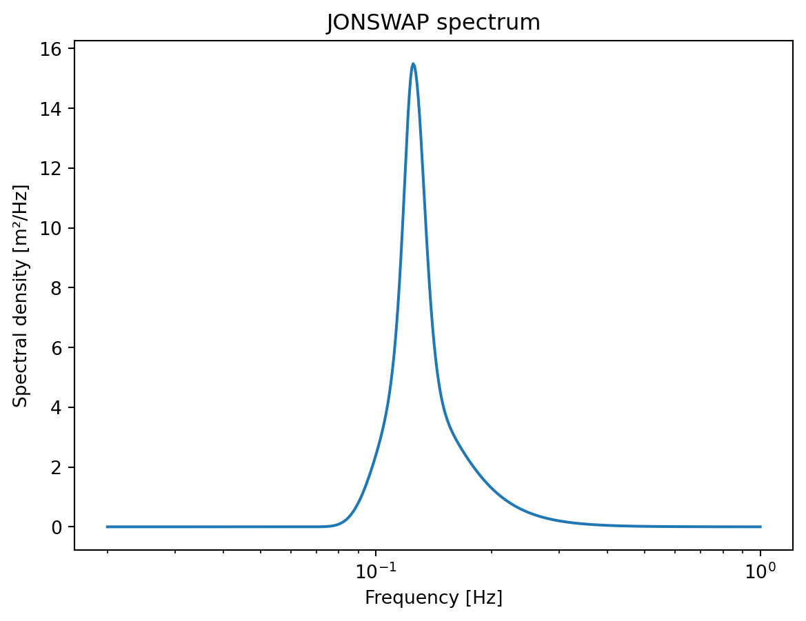
The JONSWAP spectrum (Joint North Sea Wave Project) is an empirical model that describes the distribution of wave energy across frequencies. It has a number of parameters to tune the spectrum to match measured data according to geographic position and sea state. It provides a semi-realistic method to calculate time-varying sea surface profiles for steady conditions.
4.1 The JONSWAP distribution
(Assistance for the code in this section was provided by ChatGPT.)
Code
import numpy as npimport matplotlib.pyplot as plt# Parametersg =9.81Tp =8.0# Peak period [s]fp =1/ Tp # Peak frequency [Hz]alpha =0.0081gamma =3.3# Frequency gridf = np.linspace(0.02, 1.0, 1000) # 0.02–1 Hz# Sigma switches depending on side of peaksigma = np.where(f <= fp, 0.07, 0.09)# JONSWAP spectrumr = np.exp(- (f - fp)**2/ (2* sigma**2* fp**2))S = (alpha * g**2* (2*np.pi)**-4* f**-5* np.exp(-1.25* (fp/f)**4) * gamma**r)plt.semilogx(f, S)plt.xlabel("Frequency [Hz]")plt.ylabel("Spectral density [m²/Hz]")plt.title("JONSWAP spectrum")plt.show()
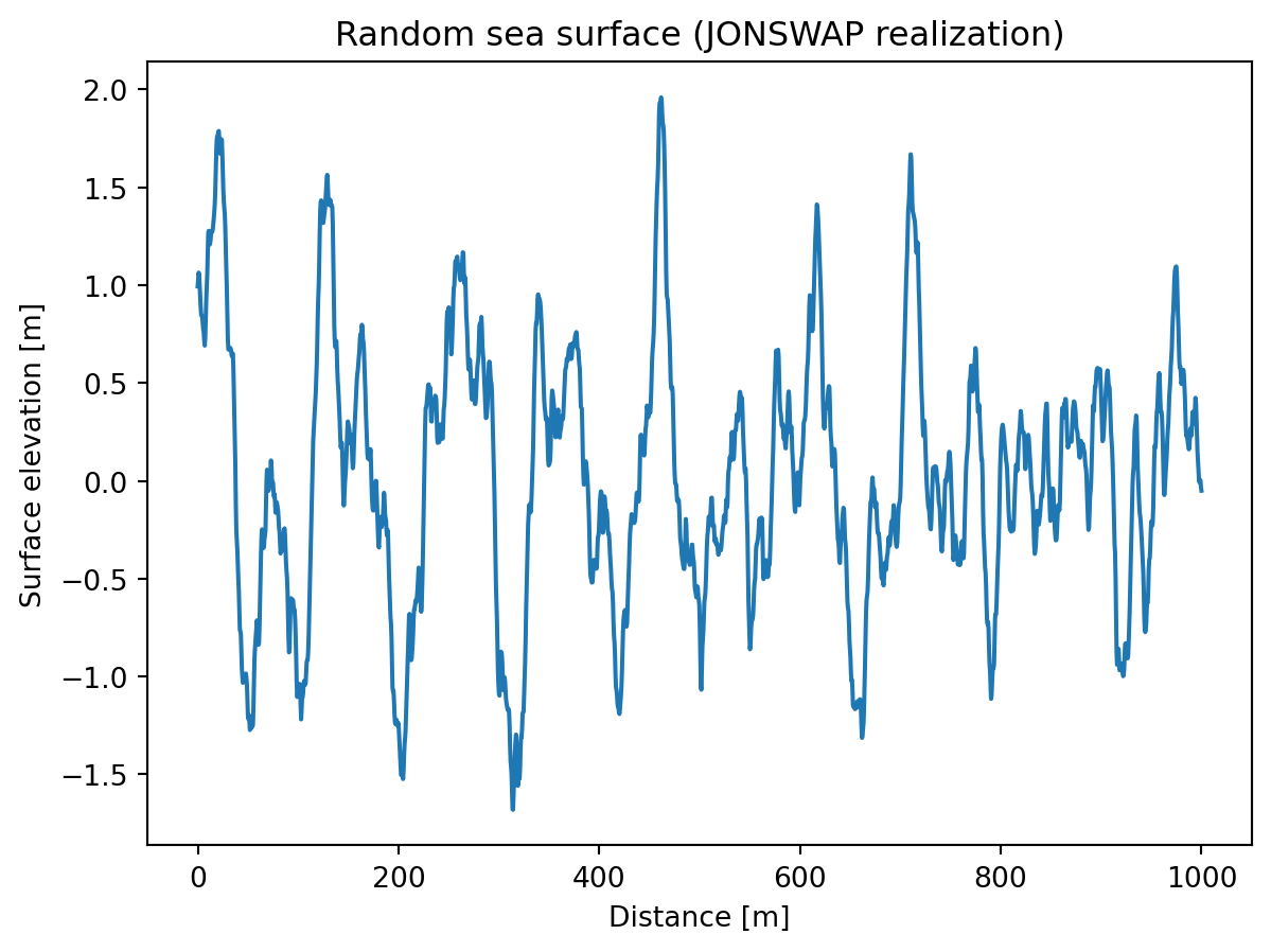
Figure 2: Time-domain synthesis of a JONSWAP surface profile.
Synthesise a time domain series:
Code
# Discretize frequencies and randomize phasesdf = f[1] - f[0]amps = np.sqrt(2* S * df)phases =2* np.pi * np.random.rand(len(f))# Convert frequency to wavenumber using deep-water dispersion: ω² = gkomega =2* np.pi * fk = omega**2/ g# Generate spatial series over your domainx = np.linspace(0, 1000, 2000) # 1000 m domaineta = np.sum(amps[:, None] * np.cos(k[:, None] * x + phases[:, None]), axis=0)plt.plot(x, eta)plt.xlabel("Distance [m]")plt.ylabel("Surface elevation [m]")plt.title("Random sea surface (JONSWAP realization)")plt.show()
Figure 3: Time-domain synthesis of a JONSWAP surface profile.
4.2 Eigenrays from JONSWAP
The distribution above can now be easily used in a Bellhop calculation:
Code
env = bh.create_env(receiver_range=200)eta = eta - np.min(eta) # ensure highest point is zeroenv["surface"] = np.column_stack((x, eta))erays = bh.compute_eigenrays(env)bhp.plot_rays(erays,env=env)
(a) Eigenrays calculated between a source and receiver with a JONSWAP sea surface profile.
(b)
Figure 4
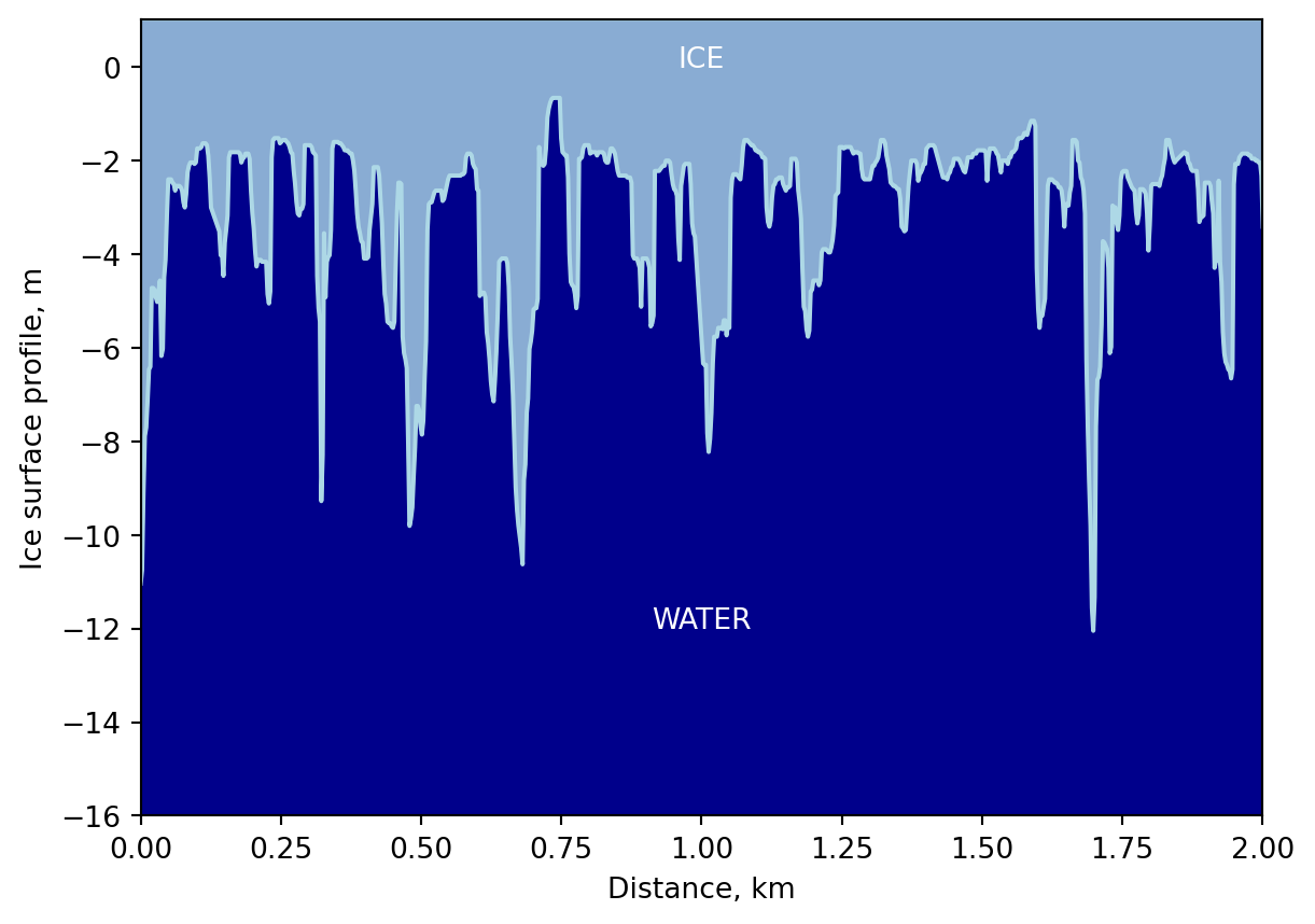
5 Sea ice surface example
The data in this example is taken from the following open access dataset (Figure 5).
National Snow and Ice Data Center. 1998, updated 2006. Submarine Upward Looking Sonar Ice Draft Profile Data and Statistics, Version 1. Boulder, Colorado USA. NSIDC: National Snow and Ice Data Center. https://doi.org/10.7265/N54Q7RWK. [Date accessed: 2025-10-09]
Code
import numpy as npimport matplotlib.pyplot as pltpath ="2000a-000b-uwa.series"withopen(path) as f: lines = f.readlines()begins = [i for i, line inenumerate(lines) if"!!! Begin !!!"in line]ends = [i for i, line inenumerate(lines) if"!!! End !!!"in line]block = lines[begins[0]+1 : ends[0]]data = np.loadtxt(block, delimiter=",")print(data[:5])dist_m = data[:,0]alti_ice = data[:,1]alti_ice = alti_ice -min(alti_ice) # ensure 0 is highest pointfig, ax = plt.subplots()ax.set_facecolor("darkblue")ax.plot(dist_m /1000, -alti_ice, color='lightblue')ax.fill_between( dist_m /1000,-alti_ice, y2=1, color='lightblue', alpha=0.8,)ax.set_xlabel("Distance, km")ax.set_ylabel("Ice surface profile, m")ax.set_xlim([0, 2])ax.set_ylim([-16, 1])ax.text(1,0,"ICE",ha="center",color="white")ax.text(1,-12,"WATER",ha="center",color="white")
(a) Underwater sea ice profile measured from upward looking sonar, data set ID G01360, file 2000a-000b-uwa.series.
(b)
Figure 5
This profile can be used to set the altimetry data in Bellhop using the surface option. For efficiency only 50 rays are shown (Figure 6). The uneven surface profile creates a complex series of reflections. A simple acousto-elastic surface boundary condition can be set up using parameters from:
Alexander, Polly and Duncan, Alec and Bose, Neil and Smith, Daniel. 2013. Modelling acoustic transmission loss due to sea ice cover. Acoustics Australia. 41 (1): pp. 79-89. https://www.acoustics.asn.au/journal/2013/2013_41_1_Alexander.pdf
Tabulated reflection coefficient data isn’t used in this example but would further increase the accuracy of the model.
Code
import bellhop as bhimport bellhop.plot as bhpice_data = np.column_stack((dist_m, alti_ice))env = bh.create_env( source_depth=20, surface=ice_data, surface_boundary_condition="acousto-elastic", surface_soundspeed=3500, surface_density=890, surface_attenuation=0.4, attenuation_units="dB per wavelength", beam_num=10, beam_angle_min=-45, beam_angle_max=45, depth=50,)erays = bh.compute_rays(env)with bhp.figure() as f: bhp.plot_rays(erays,env=env) f.xgrid.visible =False f.ygrid.visible =False
(a) A ray plot from an underwater sound source with a surface ice profile (constant depth and speed of sound).