Bellhop.py sound speed profiles

1 Depth-dependent sound speed profiles (1D)

An important consideration in underwater acoustics is the variable sound speed, which causes refraction of acoustic rays. The sound speed typically varies with depth due to changes in temperature, salinity, and pressure.

Bellhop (the executable) provides a number of interpolation routines for interpreting discretised sound speed data; some care should be used in ensuring that an appropriate interpolation is used.

Sound speed profiles can be represented in several formats. A 2xN array with the first column depths and the second column sound speeds (in m/s) is shown in Figure 1. This example shows linear interpolation. It is important to note that sound speed data is required for all depth values, so the entries must space from zero to the maximum depth of the bathymetry. In this example, a constant depth is specified (although not used until Bellhop computation occurs).

import bellhop as bh
import bellhop.plot as bhp

ssp = [[0, 1540], [10, 1530], [20, 1532], [25, 1533], [30, 1535]]
env = bh.create_env(
    soundspeed_interp="linear",
    soundspeed=ssp,
    depth=30,
)
bhp.plot_ssp(env)

Figure 1: Sound speed profile versus depth.

In the second example (Figure 2), a Pandas DataFrame is used to create a more structured sound speed profile. This format is often more useful to construct or manipulate using Pandas tools. Spline interpolation is used here. Note that the visualisation of the sound speeds shown below is performed independently in Python and further work to validate its accuracy against the Fortran code should be undertaken.

import pandas as pd
import bellhop as bh
import bellhop.plot as bhp

ssp = pd.DataFrame({
        'depth':[0, 10, 20, 30],
        'speed':[1540, 1530, 1532, 1535],
  })
env = bh.create_env(
    soundspeed_interp="spline",
    soundspeed=ssp,
    depth=30,
)
bhp.plot_ssp(env)

(a) Sound speed profile versus depth.

(b)

Figure 2

2 Interpolation types

The examples above showed soundspeed_interp="linear" and ="spline" interpolation options. The full set of options are listed in Table 1. Some description of these is provided in the environmental file documentation. Note that the A, for “analytic”, option is not provided, as this requires Fortran source code modification to function correctly.

Table 1: Bellhop sound speed interpolation options for option soundspeed_interp=. The Fortran char refers to the first digit of the “topopt” string (line 4) of the .env file.

soundspeed_interp=	Fortran char	Dimension
"spline"	S	1D
"linear"	C	1D
"pchip"	P	1D
"nlinear"	N	1D
"quadrilateral"	Q	2D — depth & range
"hexahedral"	H	3D — bellhop3D only

3 Depth- and range-dependence (2D SSP)

3.1 Loading NOAA data

Rather than cobble together artifical examples, we use the data extracted from the NOAA World Ocean Atlas by Brian Dushaw. The data has been included in the bellhop.py repository (it is not too large), and the code below adapted from Brian’s Matlab examples.

First of all load the data:

from scipy.io import loadmat

raw = loadmat("lev_ann.mat")
llz = loadmat("lev_latlonZ.mat")

ssp = 1000.0 + raw["c"] / 100.0
lat = 0.1 * llz["lat"].squeeze()
lon = 0.1 * llz["lon"].squeeze()
depth = llz["z"].squeeze()

Figure 3

Now take a lat-long slice at constant depth to visualise:

import matplotlib.pyplot as plt

lat1 = lat.reshape((360, 180), order="F")
lon1 = lon.reshape((360, 180), order="F")

depth_idx = 11
ssp1 = ssp[:, depth_idx].reshape((360, 180), order="F")

# Plot
plt.figure(figsize=(8, 4))
plt.pcolormesh(lon1, lat1, ssp1, shading="auto")
plt.colorbar(label="Sound Speed (m/s)")
plt.xlabel("Longitude (deg)")
plt.ylabel("Latitude (deg)")
plt.title(f"Sound Speed at depth ~{depth[depth_idx]} m")
plt.gca().set_aspect("equal")
plt.show()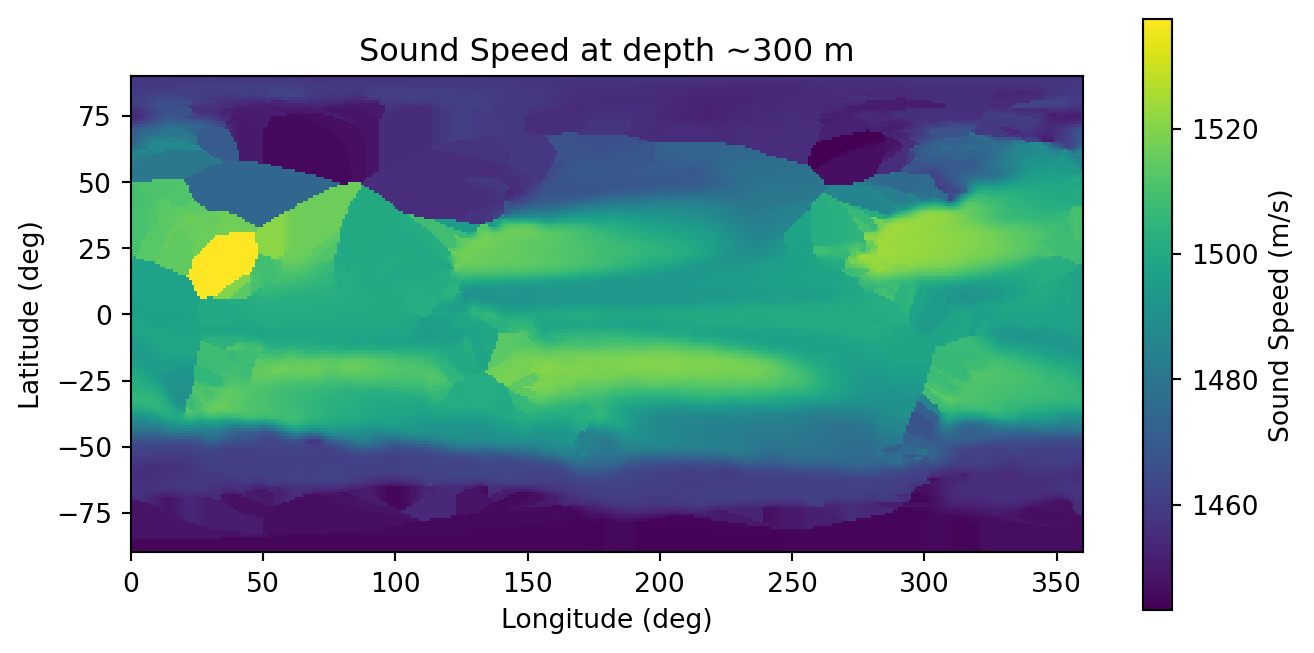

Figure 4: Worldwide sound speed profile for constant depth (NOAA World Ocean Atlas).

Now take a depth-lat slice to visualise at constant longitude:

import numpy as np

# Choose a constant longitude (e.g., 150°E)
target_lon = 200.0
lat_min, lat_max = -40, -20

# Mask points
tol = 1  # tolerance in degrees
lon_mask = np.abs(lon - target_lon) < tol
lat_mask = (lat >= lat_min) & (lat <= lat_max)
mask = lon_mask & lat_mask
ssp_subset = ssp[mask, :]
lat_subset = lat[mask]

# Sort by latitude for plotting
sorted_idx = np.argsort(lat_subset)
lat_sorted = lat_subset[sorted_idx]
ssp_sorted = ssp_subset[sorted_idx, :]

# Plot as depth vs latitude
plt.figure(figsize=(6,8))
plt.contourf(lat_sorted, depth, ssp_sorted.T, 50, cmap="viridis")
plt.gca().invert_yaxis()  # depth increases downward
plt.colorbar(label="Sound speed (m/s)")
plt.xlabel("Latitude (°)")
plt.ylabel("Depth (m)")
plt.title(f"Sound speed along longitude {target_lon}°E")
plt.show()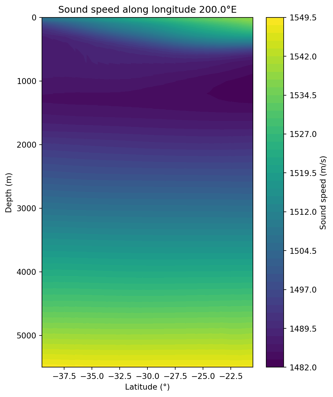

Figure 5: Worldwide sound speed profile for constant longitude (NOAA World Ocean Atlas).

Finally, convert into a Pandas DataFrame and visualise one last time in this format:

import pandas as pd

# Choose a constant longitude (e.g., 150°E)
target_lon = 200.5 # must match exactly!
lat_min, lat_max = -40, -20

# Mask points
lon_mask = np.abs(lon - target_lon) < 0.1
lat_mask = (lat >= lat_min) & (lat <= lat_max)
mask = lon_mask & lat_mask
ssp_subset = ssp[mask, :]
lat_subset = lat[mask]

# Sort by latitude for plotting
sorted_idx = np.argsort(lat_subset)
lat_sorted = lat_subset[sorted_idx]
ssp_sorted = ssp_subset[sorted_idx, :]

# 1 degree latitude ≈ 111 km
distance_km = (lat_sorted - lat_sorted[0]) * 111
svp = pd.DataFrame(ssp_sorted.T, columns=distance_km)
svp.index = depth  # distance_km from your latitude slice
plt.figure(figsize=(6,8))
plt.contourf(svp.columns, svp.index, svp, 50, cmap="viridis")
plt.gca().invert_yaxis()  # depth increases downward
plt.colorbar(label="Sound speed (m/s)")
plt.xlabel("Approx. distance (km)")
plt.ylabel("Depth (m)")
plt.title(f"Sound speed along longitude {target_lon}°E")
plt.show()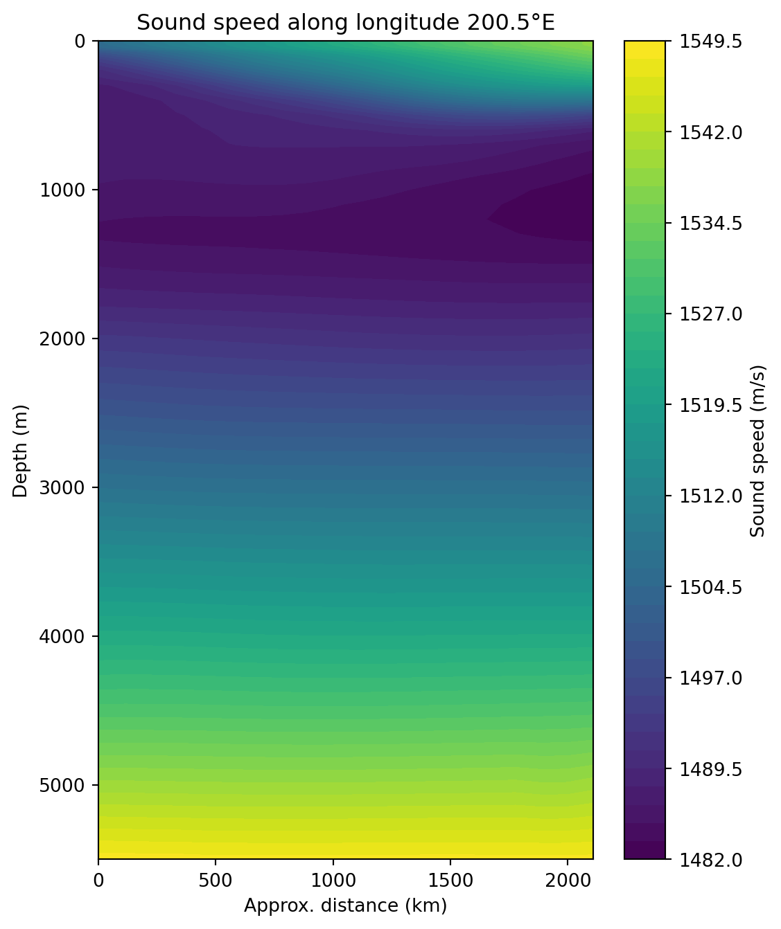

Figure 6: Worldwide sound speed profile for constant longitude (NOAA World Ocean Atlas) — converted to distance for use by bellhop.py.

3.2 2D SSP in bellhop

We are now ready to take the DataFrame created above and insert it into an appropriate environment. For a final check, plot families of SSP against range using the in-built plotting function.

import bellhop as bh
import bellhop.plot as bhp

svp.columns = distance_km * 1000.0
env = bh.create_env(
  depth=5500,
  soundspeed=svp, # see above for this 2D DataFrame definition
  soundspeed_interp="quadrilateral", # implied
  source_depth=2000,
  receiver_range=40_000,
  receiver_depth=1000,
  beam_angle_min=-89,
  beam_angle_max=89,
)
bhp.plot_ssp(env)

(a) Sound profile visualisation in 2D.

(b)

Figure 7

Based on the environment defined, we can now compute the eigenrays (Figure 8). Over such a large distance and with realistic sound speed profiles, we see some interesting nonlinear behaviour.

erays = bh.compute_eigenrays(env)
bhp.plot_rays(erays, env=env)

(a) Eigenrays calculated with a 2D sound speed profile.

(b)

Figure 8