While aubellhop takes care of all file reading and writing procedures internally, it can be useful when dealing with legacy Bellhop files or for testing different engines to be able to directly read the various files used by Bellhop.
These fall into three classes:
The environment file (.env) — special case
Supplementary input files (.ssp, .ati, .bty, .trc, .brc, .sbp) — text-based arrays of data to augment the environment file
    import aubellhop.readers as bhr
    bhr.read_ati(filename)
    bhr.read_bty(filename)

    bhr.read_brc(filename)
    bhr.read_trc(filename)

    bhr.read_sbp(filename)
    bhr.read_ssp(filename)
All six functions read in text-based BELLHOP input data and (usually) return the results in a Numpy array.
These functions are used internally by aubellhop where requested in the .env file, so their use is not generally necessary unless performing work that integrates a suite of legacy input data into a new set of simulations, or if you wish to use/visualise their data separately from running a BELLHOP simulation.
They contain columns of range and z-direction profile (“depth”) data, and optionally include five columns of geoacoustic data (compressional wave speed, compressional wave attenuation, density, shear wave speed, shear wave attenuation).
These files also specify the type of interpolation to use between data points, and therefore the reading functions have two outputs (Numpy array of data, interpolation type string).
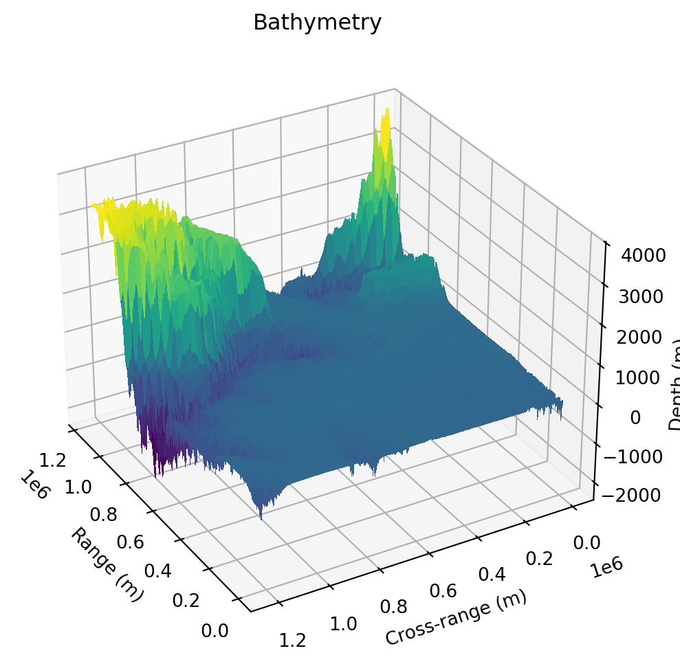
3.2 3D bathymetry
Code
import numpy as npimport aubellhop.readers as bhrimport matplotlib.pyplot as pltfrom mpl_toolkits.mplot3d import Axes3Dbty = bhr.read_bty_3d("../../examples/Bellhop3DTests/KoreanSeas/KoreanSea.bty")assert bty['depths'].shape == (721, 661)assert bty['depths'][3,4] ==-10.0assert bty['depths'][4,3] ==-50.0ranges = np.linspace(bty['ranges'][0], bty['ranges'][-1], bty['depths'].shape[0])crossranges = np.linspace(bty['crossranges'][0], bty['crossranges'][-1], bty['depths'].shape[1])depths = bty['depths'] # shape (721, 661)# Create 2D meshgridR, X = np.meshgrid(ranges, crossranges, indexing='ij') # R and X match depths shapefig = plt.figure(figsize=(12,6))ax = fig.add_subplot(111, projection='3d')# Surface plotsurf = ax.plot_surface(R, X, depths, cmap='viridis', linewidth=0, antialiased=False)ax.set_xlabel('Range (m)')ax.set_ylabel('Cross-range (m)')ax.set_zlabel('Depth (m)')plt.title('Bathymetry')ax.view_init(elev=30, azim=150) # elev = vertical angle, azim = horizontal rotation in degreesplt.show()
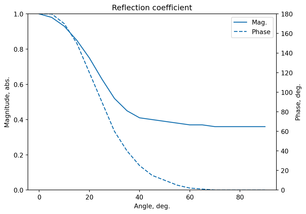
3.3 Reflection coefficient
The Acoustics Toolbox does not provide high-fidelity reflection coefficient data; the following example uses a coarse digitisation from an example in: (Figure 6.12, page 198)
Introduction to sound propagation under water
C. Erbe, A. Duncan, and K. J. Vigness-Raposa
pp. 185–216. Springer International Publishing, 2022 DOI: 10.1007/978-3-030-97540-1_6
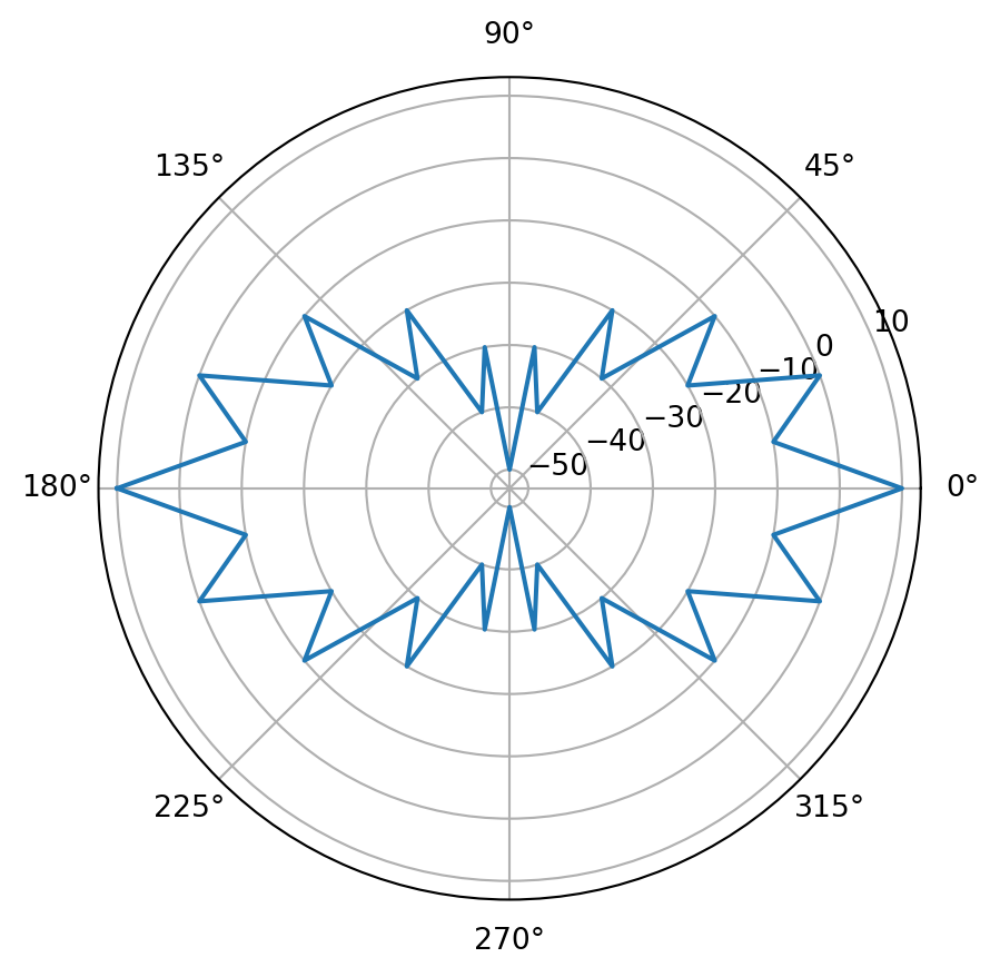
By default, sources are assumed to be omnidirectional. Source beam pattern files define directionality otherwise, stored in .sbp files (defined in the Acoustics Toolbox Bellhop guide).
These .sbp files consist of two columns: declination angle (0° is to the right, 90° is to the bottom) and dB power. The following example data is provided by the Acoustics Toolbox:
Code
import numpy as npimport matplotlib.pyplot as pltimport aubellhop.readers as bhrsbp = bhr.read_sbp("../../examples/BeamPattern/shaded.sbp")ang = sbp[:, 0] # degpow= sbp[:, 1] # dBfig = plt.figure()ax = fig.add_subplot(projection="polar")ax.plot(ang*np.pi/180, pow)plt.show()
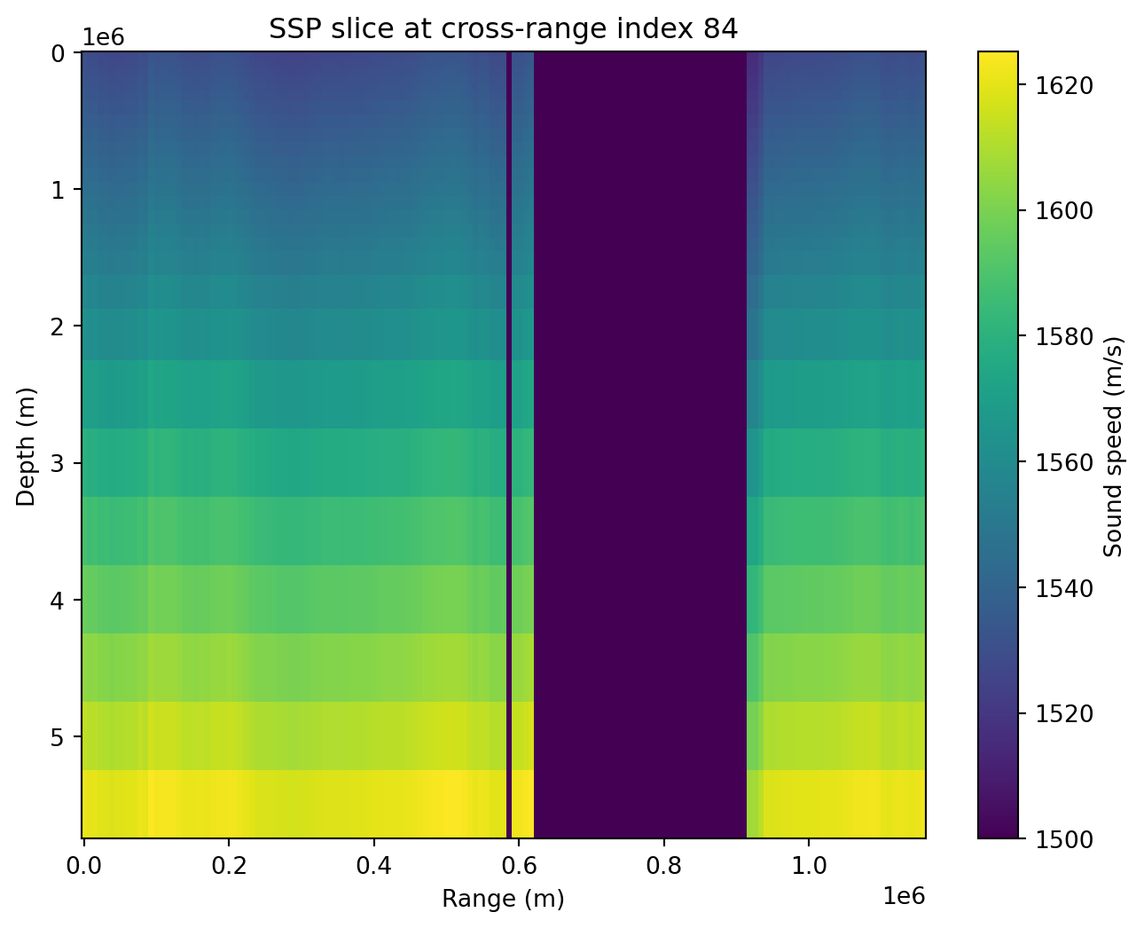
3.5 Sound speed profile (2D, 3D)
Sound speed profiles (SSPs) which vary by depth only are represented within a standard .envenvironment file. Sound speed profiles which vary by depth and range (2D), or depth and range and bearing (3D) are stored in separate .ssp text files. 3D SSP files are documented in the original BELLHOP3D user guide.
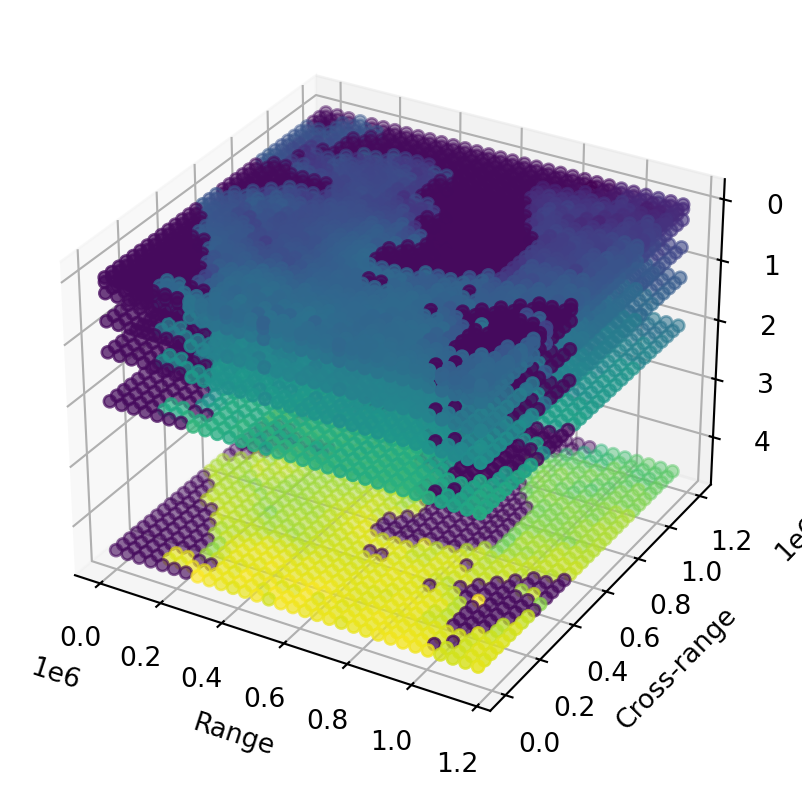
The following 3D example uses the KoreanSea.ssp data file provided with Bellhop3D; note that it has a nonuniform spacing in the z-direction (depth).
Code
import numpy as npimport matplotlib.pyplot as pltfrom aubellhop.readers import read_ssp_3dssp3d = read_ssp_3d("../../examples/Bellhop3DTests/KoreanSeas/KoreanSea.ssp")assert ssp3d["ssp"].shape == (151, 169, 33)assert ssp3d["ranges"].shape[0] ==151assert ssp3d["crossranges"].shape[0] ==169assert ssp3d["depths"].shape[0] ==33# Pick a cross-range indexcross_idx = ssp3d["crossranges"].shape[0] //2# Extract slice: depth vs range at this cross-rangessp_slice = ssp3d["ssp"][:, cross_idx, :]plt.figure(figsize=(8,6))plt.pcolormesh(ssp3d["ranges"], ssp3d["depths"], ssp_slice.T, shading='auto')plt.colorbar(label='Sound speed (m/s)')plt.xlabel('Range (m)')plt.ylabel('Depth (m)')plt.title(f'SSP slice at cross-range index {cross_idx}')plt.gca().invert_yaxis()plt.show()from mpl_toolkits.mplot3d import Axes3DR, X, Z = np.meshgrid(ssp3d["ranges"], ssp3d["crossranges"], ssp3d["depths"], indexing='ij')fig = plt.figure()ax = fig.add_subplot(projection='3d')# Take every nth point to reduce plotting sizeax.scatter(R[::5,::5,::5], X[::5,::5,::5], Z[::5,::5,::5], c=ssp3d["ssp"][::5,::5,::5], cmap='viridis', marker='o')ax.set_xlabel('Range')ax.set_ylabel('Cross-range')ax.set_zlabel('Depth')plt.gca().invert_zaxis()plt.show()
(a) Reading a .ssp text input file for a 3D sound speed profile and plotting the results.
(b)
Figure 1
4 Reading output files
The three reading functions for output files are:
    import aubellhop.readers as bhr
    bhr.read_arrivals(filename)
    bhr.read_rays(filename)
    bhr.read_shd(filename)
All three functions process a respective bellhop output file and return the results in a Pandas DataFrame. The examples below show how to work with the raw data; more convenient plotting functions are also provided via the plot or pyplot modules. Each function attempts to automatically detect whether the file it is reading is 2D or 3D, but will accept an explicit dim=2 or dim=3 argument to force the decision.
4.1 Arrivals
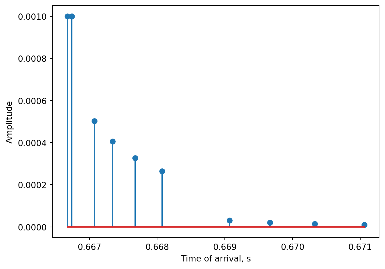
Arrivals data are stored in text-based .arr files. There are some header lines stored in the file which read_arrivals() does not output; the tabulated output data is returned in a Pandas DataFrame.
Code
import numpy as npimport aubellhop as bhimport aubellhop.readers as bhrimport matplotlib.pyplot as pltenv = bh.Environment()results = bh.compute_arrivals(env,fname_base="demo",debug=True)results_fromdisk = bhr.read_arrivals("demo.arr")# results == results_fromdiskprint("DataFrame has the following columns:")print(results_fromdisk.columns.values)plt.figure()t_arr = results_fromdisk["time_of_arrival"]arr_amp = np.abs(results_fromdisk["arrival_amplitude"])plt.stem(t_arr, arr_amp)plt.xlabel("Time of arrival, s")plt.ylabel("Amplitude")plt.show()
Using environment: bellhop/python default
Using model: [None] (default)
Using task: BHStrings.arrivals
Models found: ['bellhop']
[DEBUG] Bellhop working files NOT deleted: demo.*
DataFrame has the following columns:
<StringArray>
[       'source_depth_ndx',      'receiver_depth_ndx',
      'receiver_range_ndx',            'source_depth',
          'receiver_depth',          'receiver_range',
          'arrival_number',       'arrival_amplitude',
         'time_of_arrival', 'complex_time_of_arrival',
      'angle_of_departure',        'angle_of_arrival',
         'surface_bounces',          'bottom_bounces']
Length: 14, dtype: str
Figure 2: Reading a .arr output file and plotting the results.
4.2 Rays
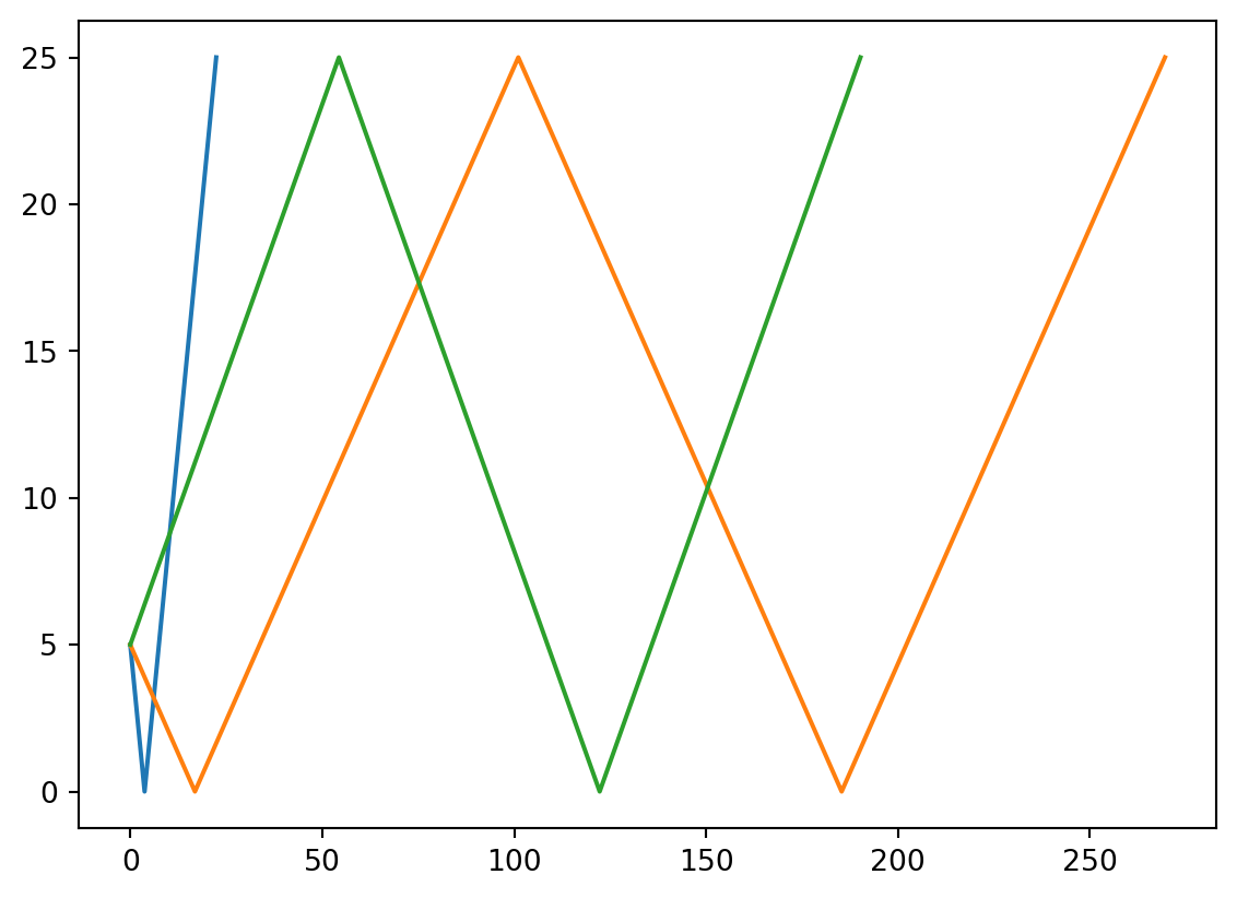
Rays data are stored in text-based .ray files. The data in these files is stored in a DataFrame with four columns:
Angle of departure (float, degrees)
Number of surface bounces (int)
Number of bottom bounces (int)
Ray trajectory coordinates (list of coordinates)
Code
import numpy as npimport aubellhop as bhimport aubellhop.readers as bhrimport matplotlib.pyplot as pltenv = bh.Environment()results = bh.compute_rays(env,fname_base="demo",debug=True)results_fromdisk = bhr.read_rays("demo.ray")print("The Nth entry of the DataFrame is:")n =12print(f"Angle of departure: {results_fromdisk.iloc[n,0]}")print(f"Number of surface bounces: {results_fromdisk.iloc[n,1]}")print(f"Number of bottom bounces: {results_fromdisk.iloc[n,2]}")print(f"Number of coordinates in the ray: {len(results_fromdisk.iloc[n,3])}")plt.figure()for n in [10,20,30]: xx = [xy[0] for xy in results_fromdisk.iloc[n,3]] yy = [xy[1] for xy in results_fromdisk.iloc[n,3]] plt.plot(xx,yy)plt.show()
Using environment: bellhop/python default
Using model: [None] (default)
Using task: BHStrings.rays
Models found: ['bellhop']
[DEBUG] Bellhop working files NOT deleted: demo.*
The Nth entry of the DataFrame is:
Angle of departure: -45.91836734693877
Number of surface bounces: 1
Number of bottom bounces: 1
Number of coordinates in the ray: 20
Figure 3: Reading a .ray output file and plotting the results.
4.3 Transmission loss
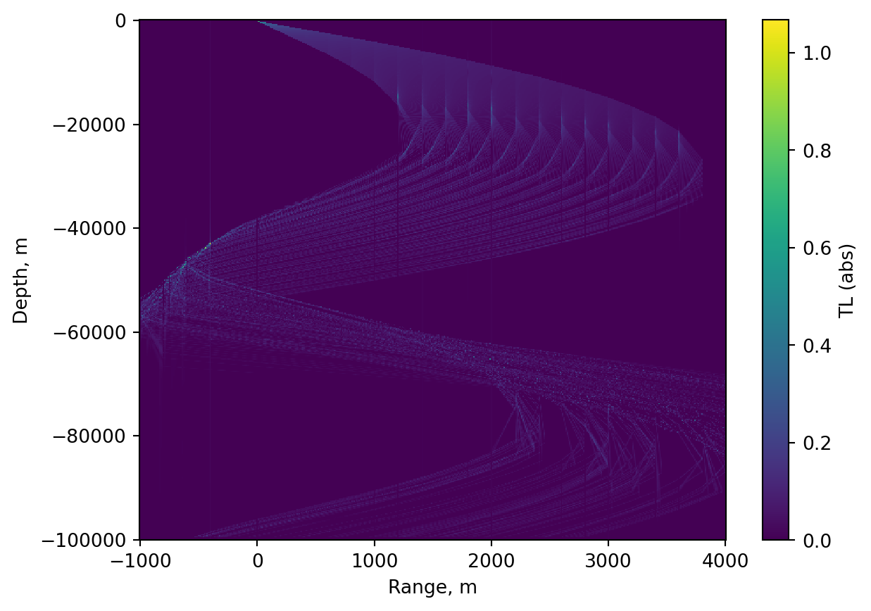
Transmission loss data are stored in binary .shd files. For gridded 2D simulations, the DataFrame is a 2D structure with column values corresponding to ranges and row index values corresponding to depths. The transmission loss data is represented as a complex value (magnitude and phase).
Code
import numpy as npimport matplotlib.pyplot as pltfrom aubellhop.readers import read_shddf = read_shd("../../tests/MunkB_geo_rot/MunkB_geo_rot.shd")X, Y = np.meshgrid(df.columns.values, df.index.values)Z1 = df.valuesplt.figure()plt.pcolormesh(X, Y, abs(Z1), shading='nearest')plt.colorbar(label='TL (abs)')plt.xlabel('Range, m')plt.ylabel('Depth, m')plt.show()
Figure 4: Reading a .shd binary output file and plotting the results.